Random
 Collection
114 standalone TikZ figures, mostly about , , .
MIT licensed (free to reuse) Repo
Have a TikZ image you'd like to share with attribution?
Submit a PR with a standalone .tex file
and metadata .yml file to add it to this list.
Autoencoder
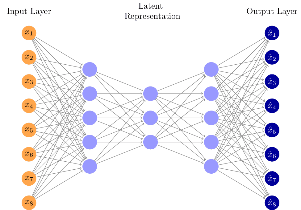
Variational autoencoder architecture. Made with https://github.com/battlesnake/neural.
Aviary

Aviary logo: a repo of machine learning models for representation learning in materials discovery from stoichiometry and symmetries via graph convolutions. For https://github.com/CompRhys/aviary.
Basis + Lattice
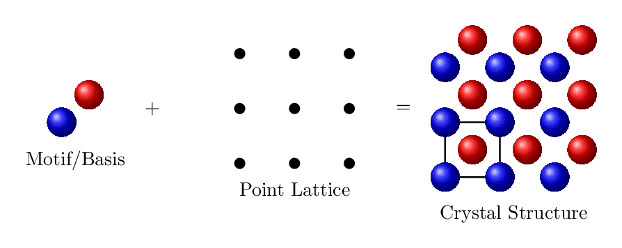
Operation illustrating combination of a motif/basis with a point lattice to generate a crystal structure.
Bloch Sphere
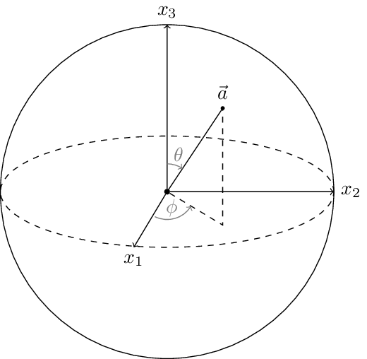
A Bloch sphere of radius |a| = 1 contains all possible states of a two-state quantum system (qubit). Each Bloch vector fully determines a spin-1/2 density matrix. Used in Exercise Sheet 10 of Statistical Physics by Manfred Salmhofer (2016), available at https://janosh.dev/physics/statistical-physics.
Bose Einstein Distribution
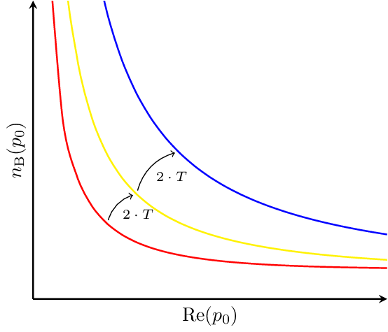
Illustrating the change in the real part of the Bose-Einstein distribution, i.e. the average occupancy of the ground state of a bosonic system, from doubling the temperature. Pulled from arxiv:1712.09863.
Bose Einstein Distribution 3d
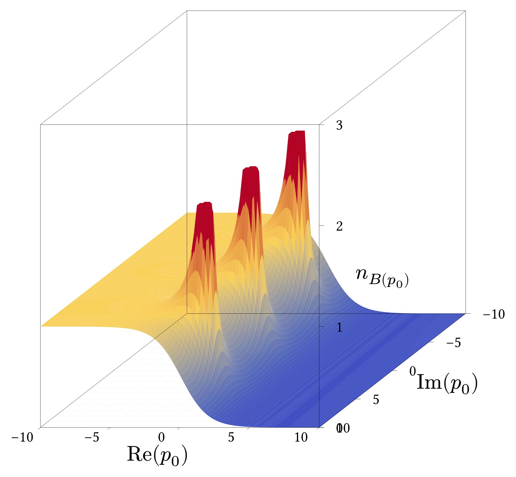
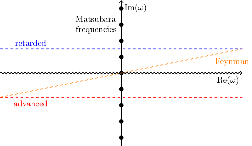
Surface plot of the Bose-Einstein distribution over the complex plane. This plot shows an important feature of the Matsubara formalism developed for QFT at non-zero temperature. It's a method to calculate expectation values of operators in a canonical ensemble evolved by an imaginary time. In momentum space, this leads to the replacement of continuous frequencies by discrete imaginary (Matsubara) frequencies. Away from the imaginary axis, the distribution becomes approximately flat, particularly at sufficiently low temperatures. Pulled from arxiv:1712.09863.
Branch and Bound
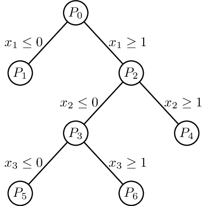
Illustration of a linear-programming (LP)-based branch and bound algorithm. Not knowing how to solve a mixed-integer programming (MIP) problem directly, it first removes all integrality constraints. This results in a solvable LP called the linear-programming relaxation of the original MIP. The algorithm then picks some variable x restricted to be integer, but whose value in the LP relaxation is fractional. Suppose its value in the LP relaxation is x = 0.7. It then excludes this value by imposing the restrictions x ≤ 0 and x ≥ 1, thereby creating two new MIPs. By applying this recursively step and exploring each resulting bifurcation, the globally optimal solution satisfying all constraints can be found.
Branch Cuts 1

Propagator branch cuts, i.e. a continuum of singularities, along the real frequency axis extending from out to . Pulled from arxiv:1712.09863.
Branch Cuts 2
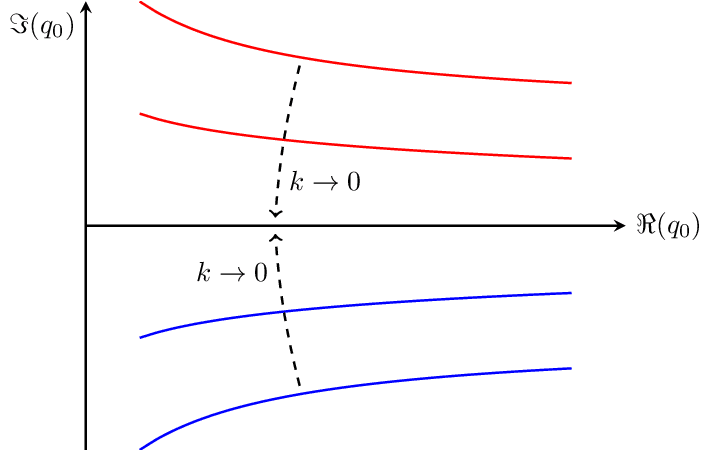
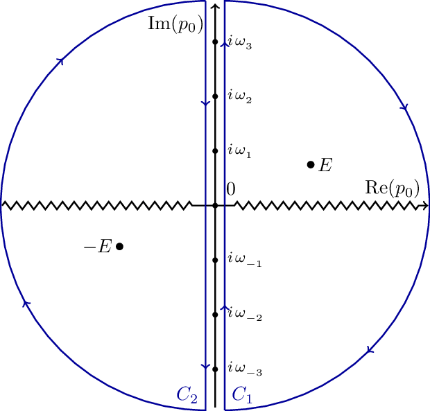
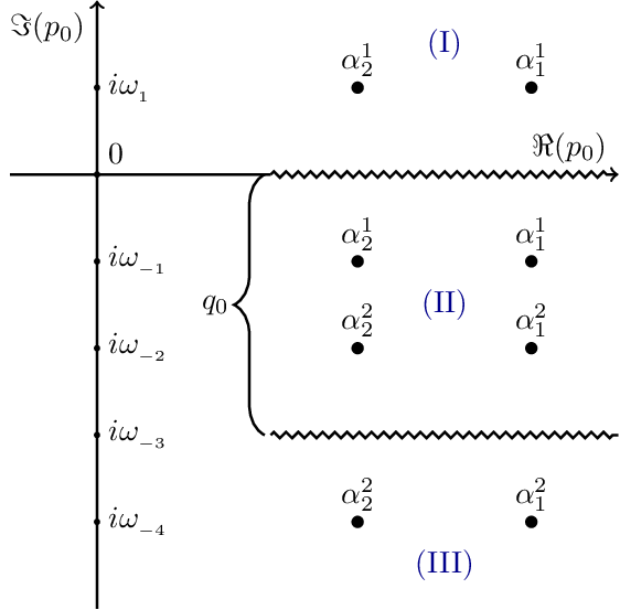
Branch cuts approaching the real -axis with decreasing where they merge at . denotes the energy cutoff of a scalar field theory.
Change of Variables
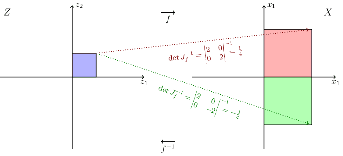
Simple 2d example illustrating the role of the Jacobian determinant in the change of variables formula. Inspired by Ari Seff in https://youtu.be/i7LjDvsLWCg?t=250.
Closed String Topologies
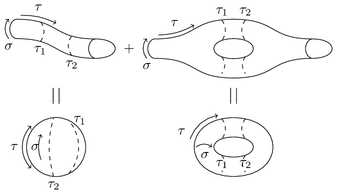
When calculating scattering amplitudes via the path integral, we must sum over all possible world-sheet topologies. To characterize the types of world-sheets that have to be considered at each level of its perturbative expansion, string theory makes use of the following theorem:
Every compact, connected, oriented two-dimensional manifold is topologically equivalent to a sphere with handles ( for genus) and boundaries. A topological invariant of two-dimensional oriented surfaces is the Euler characteristic .
What this boils down to is that we can obtain the topological characteristics of higher and higher loop-level world-sheet topologies by successively increasing in one-step increments the number of handles in case of the closed string and the number of boundaries for the open sector. This gives the topologies in this figure for the vacuum diagram of the closed sector up to one-loop level. For the open sector, see open string topologies.
Common Activation Functions in Machine Learning
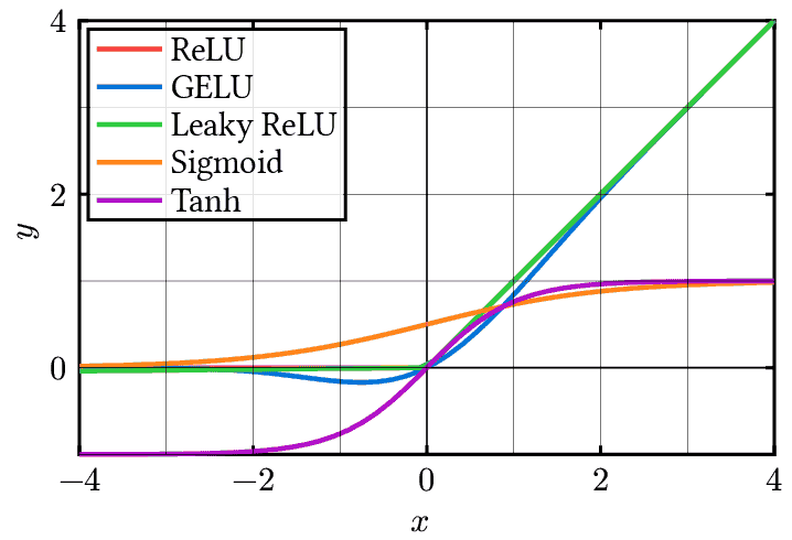
Plot of common machine learning activation functions. Includes the Rectified Linear Unit (ReLU), Gaussian Error Linear Unit (GELU), Leaky ReLU, Sigmoid, and Hyperbolic Tangent (tanh) activation functions. Activation functions introduce non-linearity into neural networks, enabling them to learn complex patterns and relationships in data. The choice of activation function can have a significant impact on the performance and convergence of a neural network. ReLU is widely used due to its simplicity and ability to alleviate the vanishing gradient problem. GELU and Leaky ReLU are variants of ReLU that address some of its limitations. Sigmoid and tanh are classical activation functions that squash the input to a fixed range, but they are less commonly used in modern deep learning architectures due to the vanishing gradient problem.
Complex Sign Function
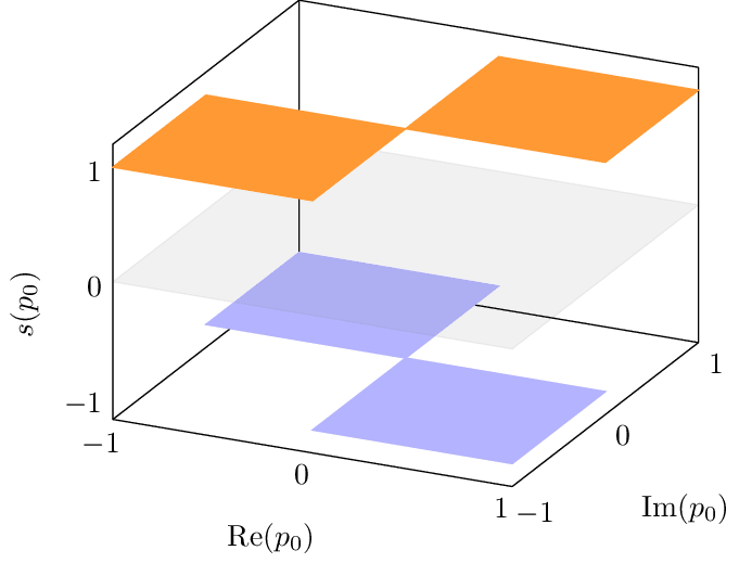
3d surface plot of the complex sign function over the complex plane. Used in the Matsubara summation of thermal quantum field theory to split contour integrals in the complex plane into two parts, the first being branch-cut free and the second evident branch cut structure.
Concave Functions
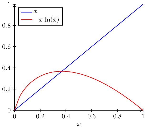
is convex and is its tangent, so .
Contour Deformation

Conv2d
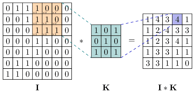
A two-dimensional convolution operator slides the kernel matrix across the target image and records elementwise products. Makes heavy use of the matrix environment in TikZ.
Convex Functions
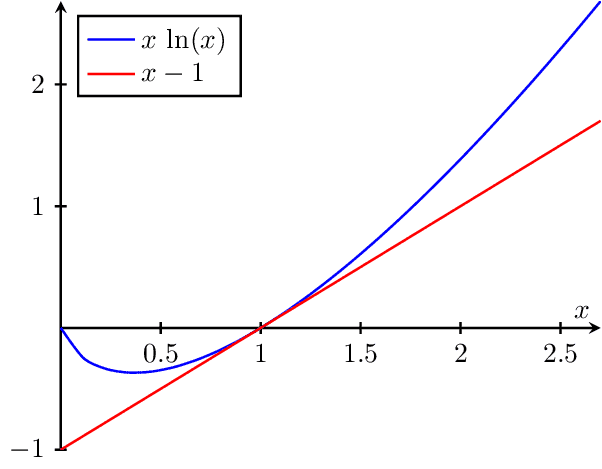
and are concave functions. Since decomposes into sums of these two components, it too must be concave. Any extremum of a concave function is a maximum. This fact is used in statistical physics to find the equilibrium distribution of many-particle systems. See problem 2 on this exercise sheet.
Convex Hull of Stability
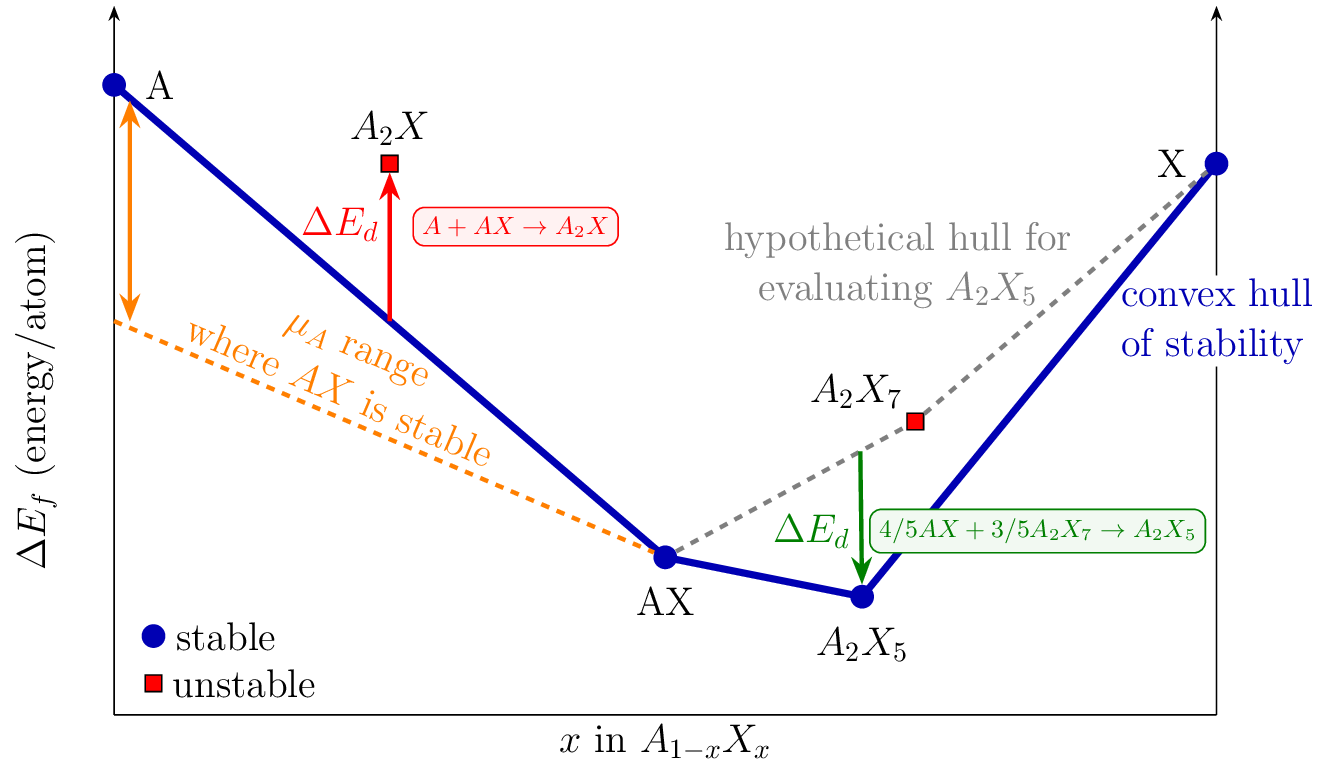
Reproduced from Bartel et al. http://dx.doi.org/10.1007/s10853-022-06915-4. The convex hull of stability represents the lowest energy surface in composition space for a given chemical system. It is constructed by connecting the energies of the most thermodynamically stable compounds at each composition. For visual clarity, only ground-state phases at each composition are shown. Legend:
- Blue circles: Stable phases lying on the convex hull (blue line)
- Red squares: Unstable phases above the hull
- Orange dashed line: Chemical potential range where AX is stable
- ΔE_d: Decomposition enthalpy, the energy above the hull for unstable phases
Materials on the hull are stable against decomposition into other phases. The energy difference between a material and the hull (hull distance) quantifies its thermodynamic stability - larger distances meaning less stable and harder to synthesize, making the convex hull a powerful tool for guiding experimental synthesis efforts.
Cost vs Accuracy in Quantum Mechanics Simulations
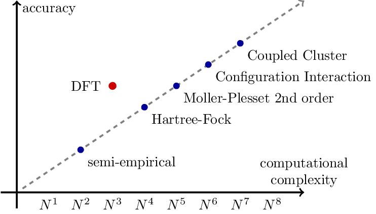
Cost vs accuracy trade-off for different quantum mechanics approximations. denotes the system size, usually the number of electrons. Source: Frank Noe.
Cylinder to Plane
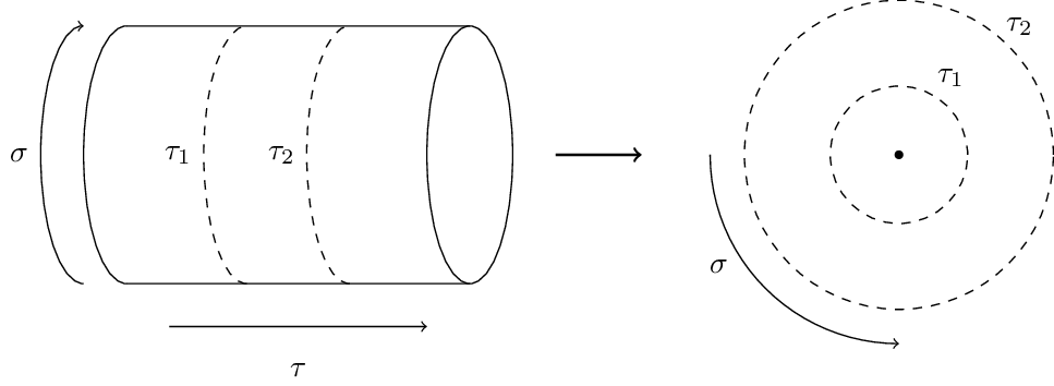
String theory: Primary fields and radial quantization A time-ordered product of fields on the cylinder maps to a radially ordered product in the complex plane. This graphic visualizes how different times on the cylinder correspond to different times on the plane.
Diagrams

Disk to Plane
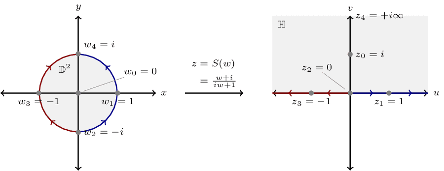
Divergence
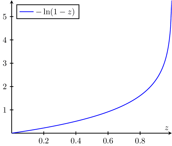
Plot of which diverges at .
Dropout
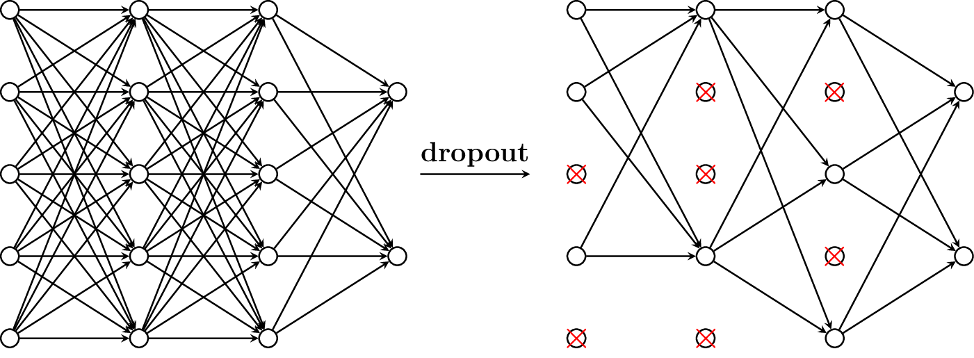
Illustration of applying dropout with a rate of to a multilayer perceptron.
Ergodic
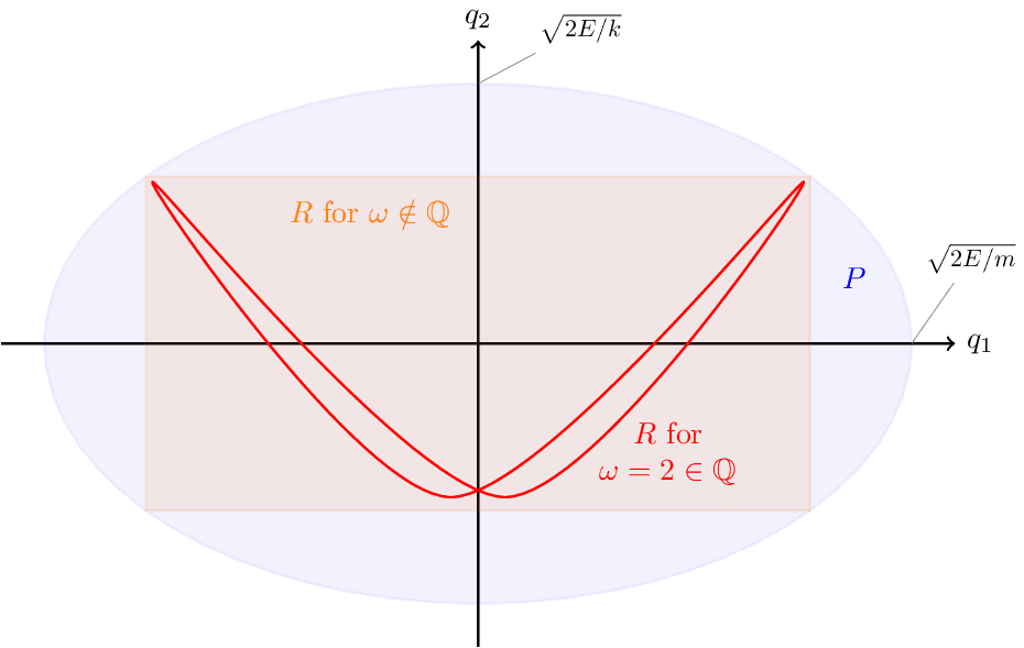
Euler Angles
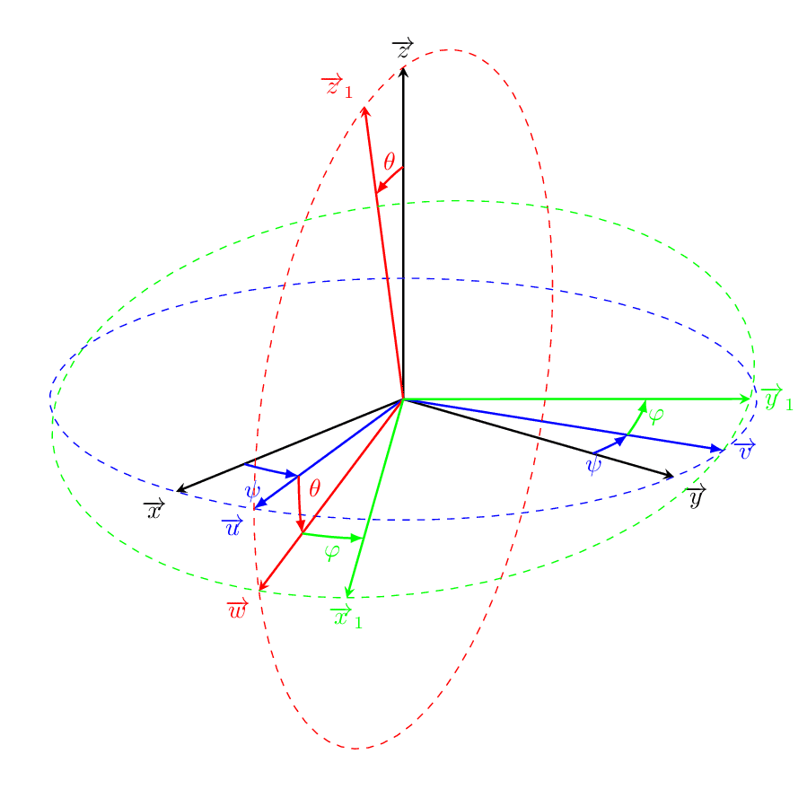
Named after the mathematician Leonhard Euler, the 3 Euler angles describe arbitrary orientations in 3d w.r.t. to some coordinate system. They can also represent the orientation of a frame of reference in physics or of a general basis in 3d linear algebra.
Fermi-Dirac Distribution
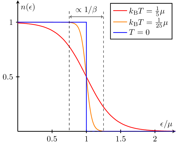
A plot illustrating the Fermi-Dirac distribution function for different temperatures relative to the chemical potential (). The plot demonstrates how the occupation number () changes as the temperature increases from zero to higher values. The visualization also highlights the effect of thermal fluctuations, which increase with higher temperatures.
Ferroelectric Response
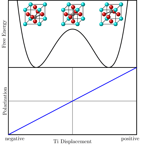
Schematic representation of ferroelectric response for BaTiO3 depicting the double-well free energy potential and polarization plots. The figure illustrates the movement of the Titanium atom within the crystal lattice as it shifts between two stable positions, corresponding to minima in the free energy curve. This Titanium displacement results in a large change in the material's polarization.
Feynman 1

Feynman 2

Feynman 3
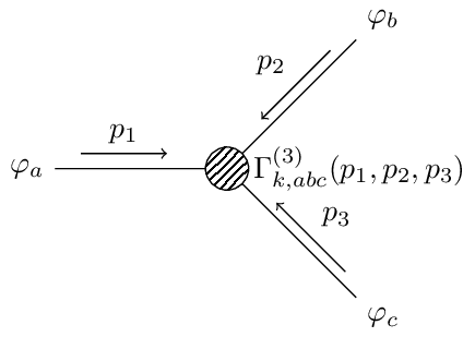
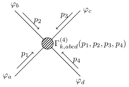
Feynman 4
Feynman Diagram Propagator Loop
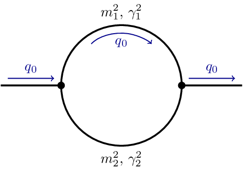
This Feynman diagram contains two propagators forming a loop carrying the external energy . denote the masses of the propagators and their decay width which, for an expansion in Minkowski space, are non-zero only around a real and positive on-shell frequency .
Fluctuations
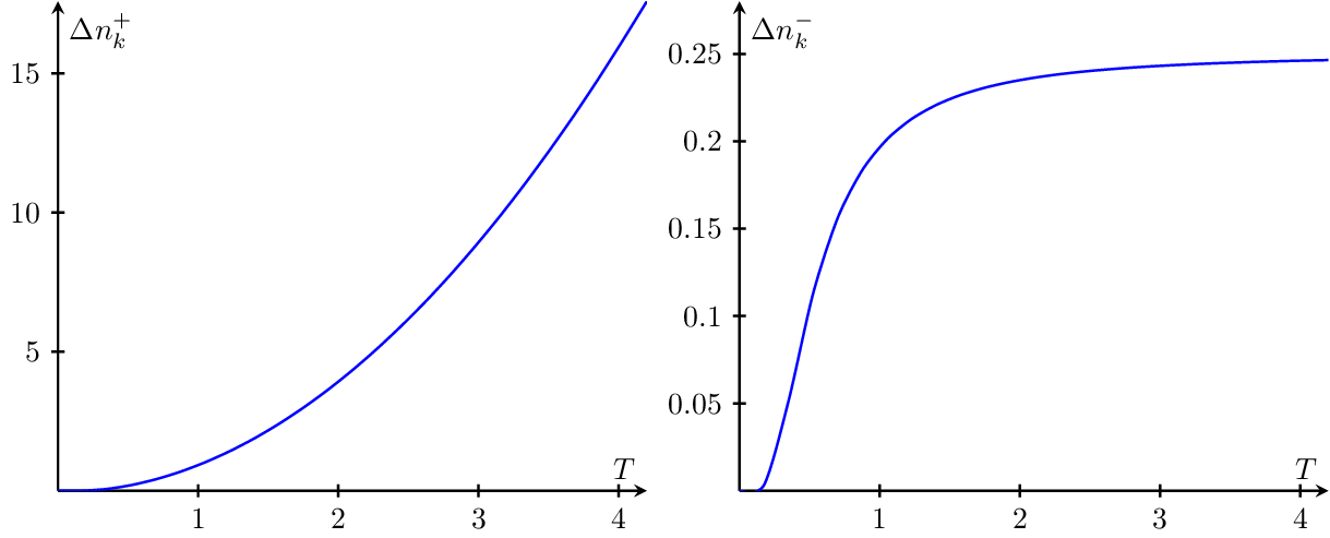
Number fluctuations of the occupation probability〈nk〉of a single mode k in an ideal Bose and Fermi gas in the grand canonical ensemble. Used in Exercise Sheet 11 of Statistical Physics by Manfred Salmhofer (2016), available at https://janosh.dev/physics/statistical-physics.
Four Vs of Data
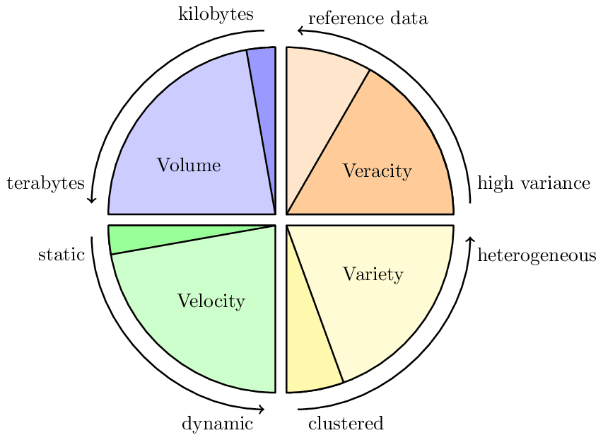
The state of the 4 Vs of data as they apply to materials informatics. Inspired by fig. 1 in https://api.semanticscholar.org/CorpusID:137734316.
GAN

Generative adversarial network (GAN) architecture. A GAN has two parts. The discriminator acts as a classifier that learns to distinguish fake data produced by the generator from real data. incurs a penalty when detects implausible results. This signal is backpropagated through the generator weights such that learns to produce more realistic samples over time, eventually fooling the discriminator if training succeeds.
Geometric Bayes
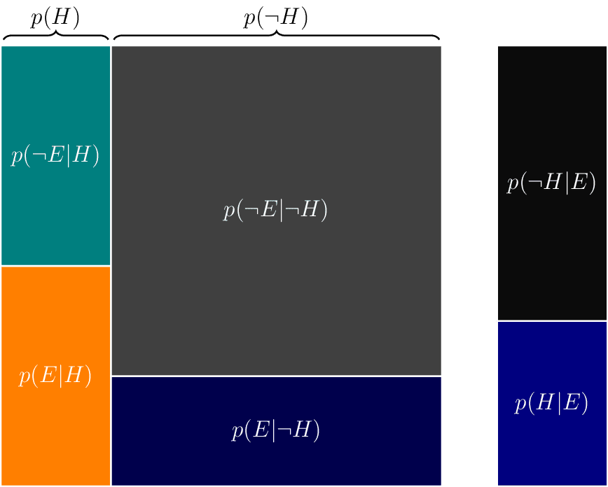
3blue1brown-inspired geometric visualization of Bayes theorem https://youtu.be/HZGCoVF3YvM.
Graph Isomorphism

Graphs can look differently but be identical. The only thing that matters are which nodes are connected to which other nodes. If there exists an edge-preserving bijection between two graphs, in other words if there exists a function that maps nodes from one graph onto those of another such that the set of connections for each node remain identical, the two graph are said to be isomorphic.
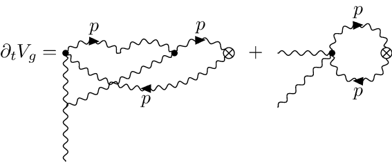
Gravitons
Harmonic Oscillator Energy vs Angular Frequency
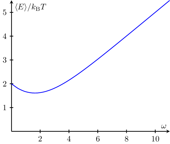
Harmonic oscillator energy vs angular frequency
Harmonic Oscillator Energy vs inverse Temperature
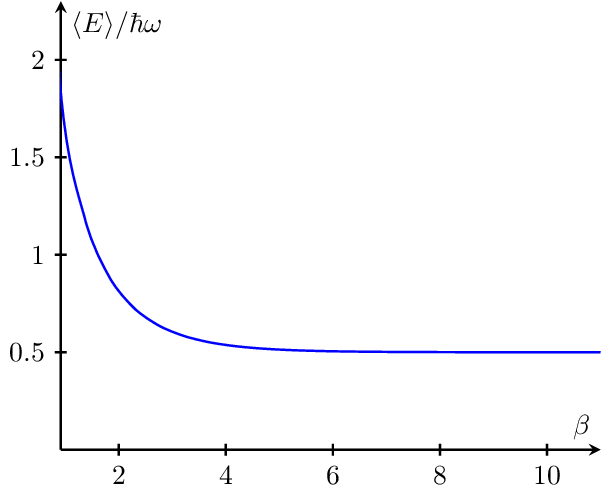
Harmonic oscillator energy vs inverse temperature beta = 1/(kB T)
Heatmap
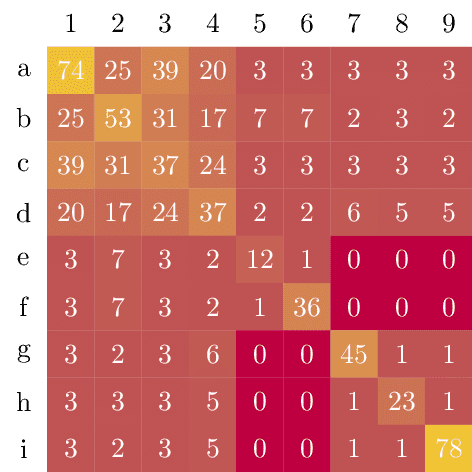
Posted as an answer to https://tex.stackexchange.com/q/44868.
Higgs Potential
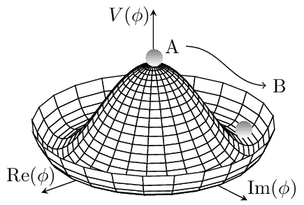
The Higgs mechanism plays a vital role in the Standard Model for explaining how gauge bosons obtain mass. The Standard Model would otherwise predict these particles to be massless. Through interactions with the Higgs field that permeates all space and whose elevated potential at zero field leads to spontaneous symmetry breaking (SSB), gauge bosons also experience symmetry breaking, causing them to acquire mass. See https://janosh.github.io/tikz/maxican-hat for a very similar image.
High Entropy Alloy

Cartoon of the AlCoCrFeNi high entropy alloy (HEA) with body-centered cubic (BCC) lattice. HEAs also come in face-centered cubic (FCC) and (less frequently) hexagonal close packing (HCP). BCC HEAs typically have high yield strength and low ductility, vice versa for FCC HEAs. Wiki article.
Identical Particle Energy Distribution Function Comparison
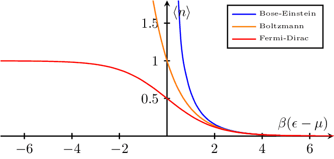
A plot comparing the distribution functions of Bose-Einstein, Boltzmann, and Fermi-Dirac statistics as a function of the reduced chemical potential . This visualization highlights the differences between the three types of distribution functions, which are used to describe the behavior of particles in different statistical systems.
Isotherms
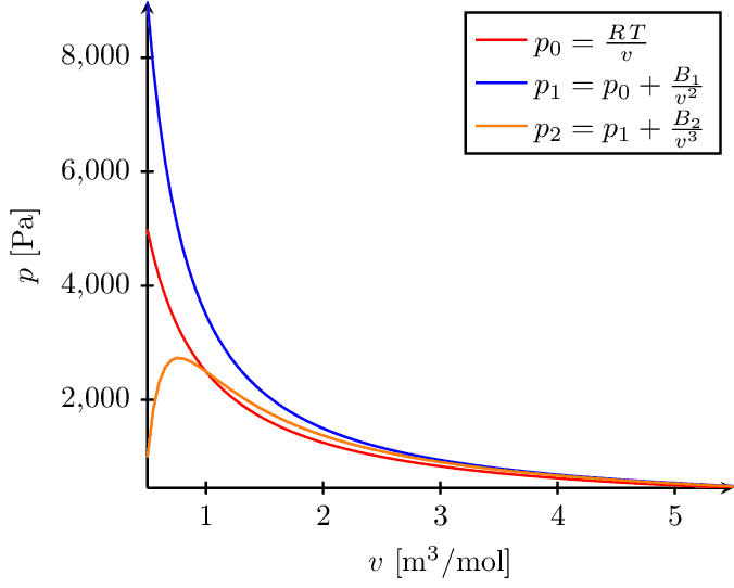
This image visualizes the behavior of gas isotherms (curves showing pressure-volume relationships at constant temperature), represented by three equations of state, as a function of volume. The equations include the ideal gas law, and two other modified laws accounting for molecular interactions. The x-axis represents the molar volume and the y-axis represents the pressure of the gas.
Jensens Inequality
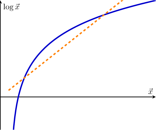
This graph illustrates Jensen's Inequality, a fundamental concept in mathematical optimization and probability theory. It compares a convex function (blue curve, representing the natural logarithm function) with a linear function (orange dashed line). The inequality states that for a convex function, the function of an expectation is always less than or equal to the expectation of the function, depicted here by the fact that the dashed line is always above the curve. Equality holds if and only if the random variable is a constant (i.e. there is no randomness).
k-Space
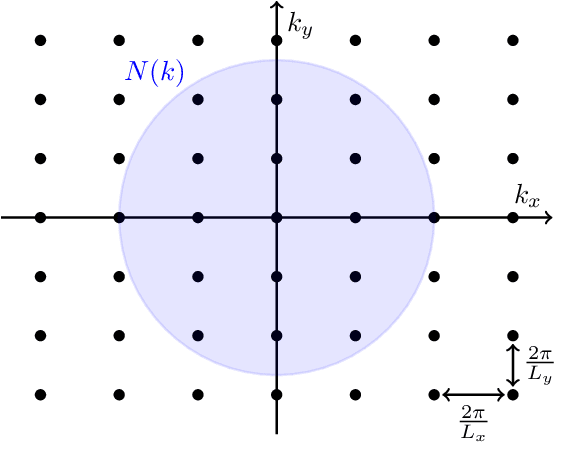
The -space region of wave vectors up to a given magnitude is a disk of area . The -space area occupied by a single particle state is
where the factor of is due to the spin degeneracy . The number of states with wave vector magnitude smaller than is
-space is used extensively in solid state physics e.g. to visualize the energy bands of a material as a function of electron momentum. In position space, the position-energy dispersion would just be a probability blur.
Kohn Sham Cycle
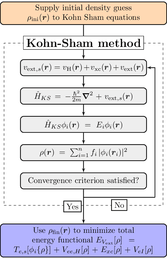
This diagram illustrates the Kohn-Sham cycle in Density Functional Theory (DFT), a computational quantum mechanical modeling method. The process starts with an initial guess for the electron density, which is used to calculate the effective potential. This potential is then used in the Kohn-Sham Hamiltonian, which is solved to obtain the wavefunctions. These wavefunctions are used to compute a new electron density. If convergence criteria are met, the final electron density is used to calculate the total energy functional. If not, the new electron density is used for the next iteration of the cycle.
Kohn-Sham DFT User Choices
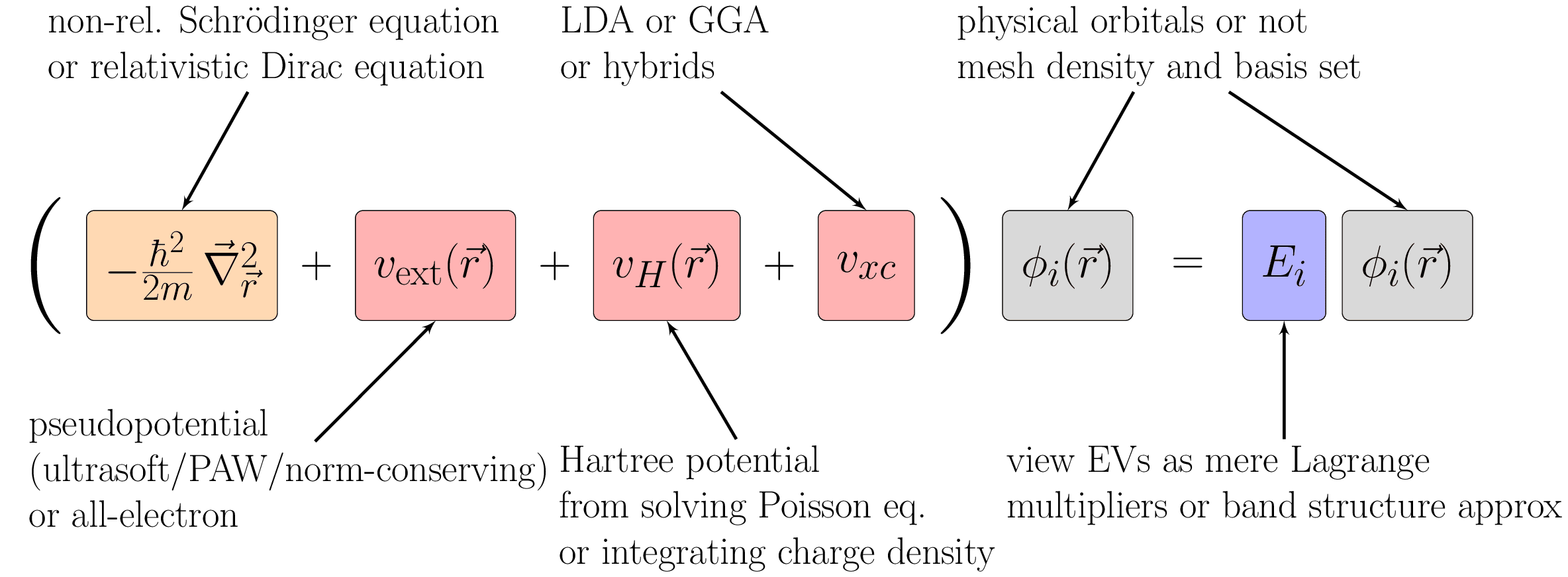
Visualization of the many choices involved in a Kohn-Sham calculation. It can be non-relativistic based on the classical Schrödinger equation or fully relativistic based on the Dirac equation which includes spin-orbit coupling. The near-core electrons can be modeled explicitly in an all-electron calculation or, much more commonly, incorporated along with the nucleus into an effective pseudo-potential. The Hartree energy can be obtained by integrating the charge density or by solving the Poisson equation. The exchange-correlation potential can be treated with a huge library of density functionals, most commonly LDA and GGA. The wave functions can be computed on a numerical mesh and expanded in one of many possible basis sets, e.g. plane waves, APW, or PAW. Inspired by fig. 3 in arxiv:cond-mat/0211443.
Loop
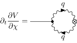
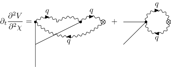
Loops
M-Theory
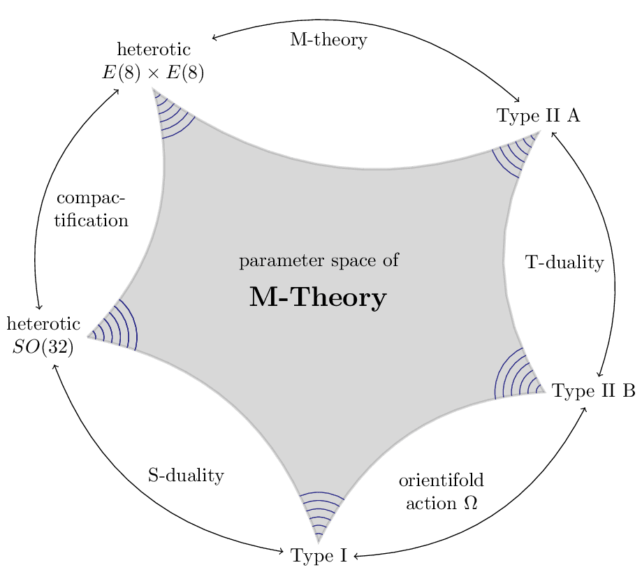
One of the pivotal insights of the 2nd superstring revolution point was Edward Witten's formulation of M-Theory in 1995. Before that, there had been 5 different types of string theories, each 10-dimensional: Type I, Type IIa and IIb, and two different heterotic theories. Witten showed that all of these theories are simply different limiting cases of a single overarching string theory (without showing what that underlying theory actually is). See Sean Carroll's excellent post on M-Theory for details.
MADE
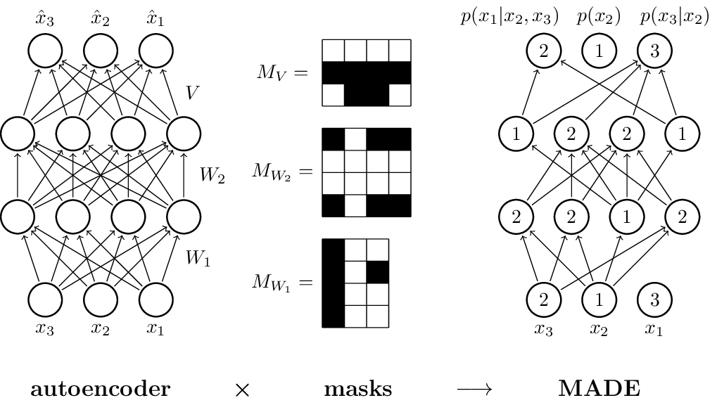
TikZ-reproduction of fig. 1 from the paper MADE: Masked Autoencoder for Distribution Estimation (arxiv:1502.03509).
MAF
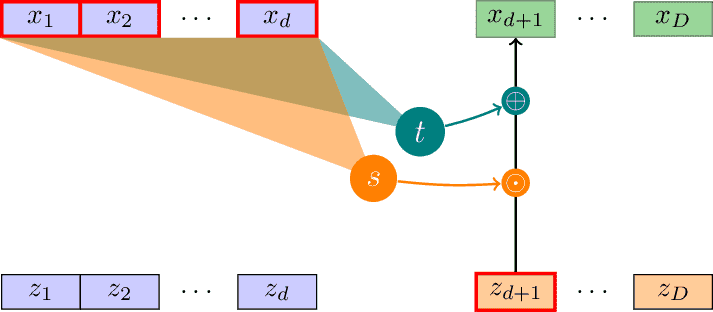
Illustration of the slow (sequential) forward pass of a Masked Autoregressive Flow (MAF) layer as introduced in arxiv:1705.07057. Inspired by https://blog.evjang.com/2018/01/nf2.html.
Materials Informatics

Structure-based materials informatics workflow. Inspired by fig. 1 in https://doi.org/10.1016/j.cpc.2019.106949.
Materials Informatics Challenges

Inspired by https://tex.stackexchange.com/a/387466.
Matsubara Contour 1
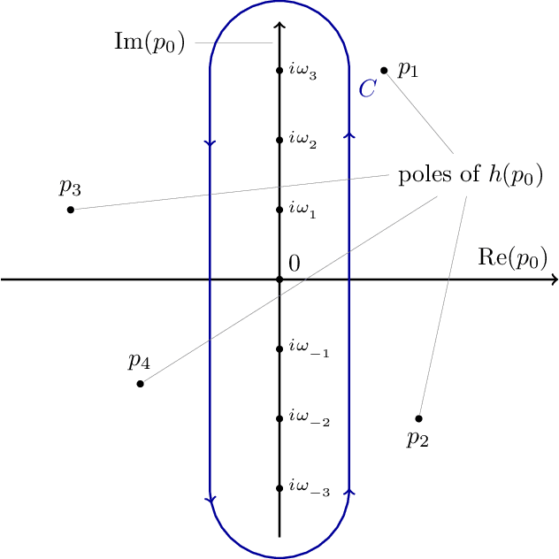
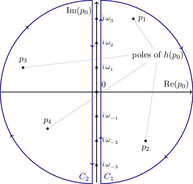
Complex contour plot illustrating a Matsubara summation. Used in thermal quantum field theory to compute Feynman diagrams at non-zero temperature. surrounds the imaginary -axis counterclockwise but excludes poles of .
Matsubara Contour 2
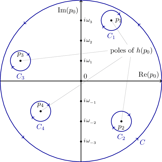
Deformation of contour in Matsubara contour 1 into a circle followed by taking the radius to infinity. This will enclose the poles of scattered throughout the complex plane. Their contribution is removed again by enclosing them in clockwise contours.
Matsubara Contour 3
Matsubara Contour 4

Matsubara Contour 5
Maxwell Boltzmann Distribution
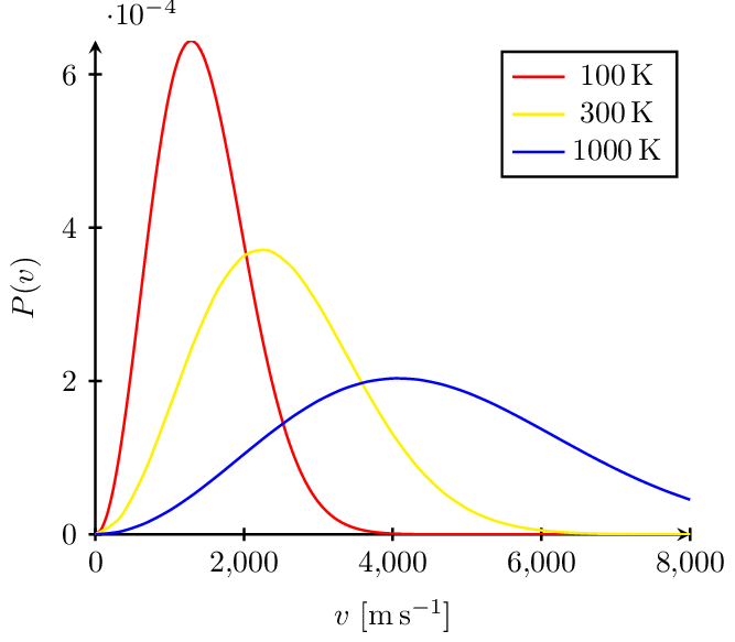
The Maxwell-Boltzmann distribution plotted at different temperatures reveals that the most probable velocity of ideal gas particles scales with the square root of temperature.
Mexican Hat
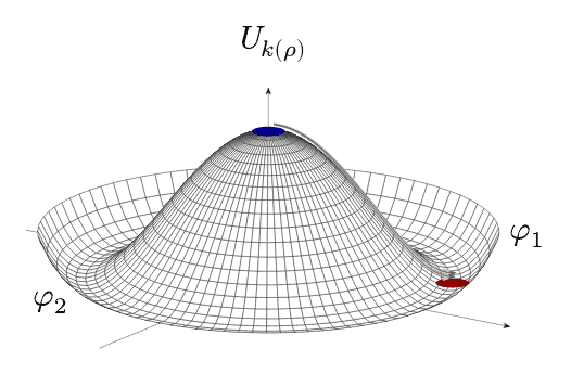
The Mexican hat potential exhibits spontaneous symmetry breaking (SSB), a process by which a physical system starting in a symmetric state spontaneously enters and remains in an asymmetric state. This usually applies to systems whose equations of motion obey a set of symmetries while the lowest-energy state(s) do(es) not. When the system assumes one of its ground states, its symmetry is broken even though the Lagrangian as a whole retains it. See https://janosh.github.io/tikz/higgs-potential for a very similar image.
In this image, the system starts out in the naive -invariant vacuum (blue dot) but quantum fluctuations quickly push it into the real vacuum (red dot) where is broken down to .
MOSFET
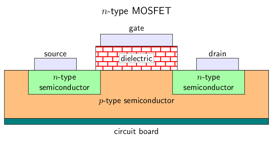
The metal-oxide-semiconductor field-effect transistor, or MOSFET for short, is the most frequently manufactured device in history, with close to 10^23 MOSFETs produced since 1960. As the basic building block of almost all modern electronics, it revolutionized the world economy and triggered our ascent into the information age.
Mphil Gantt
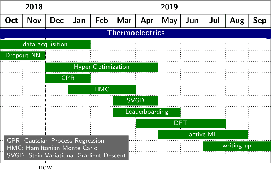
Useless Gantt chart for my Scientific Computing MPhil project at Cambridge University titled "Data-Driven Risk-Conscious Thermoelectric Materials Discovery". See https://github.com/janosh/thermo.
NF Coupling Layer

Simple 2d example illustrating the role of the Jacobian determinant in the change of variables formula. Inspired by Ari Seff in https://youtu.be/i7LjDvsLWCg?t=250.
Normalizing Flow

A chain of bijections constituting a normalizing flow which step by step transforms a simple distribution into a complex one . The bijections are trained to fit to some target distribution . Inspired by Lilian Weng.
One Point
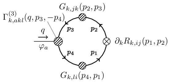
This Feynman diagram corresponds to the integrand in this expression for
Open String Topologies
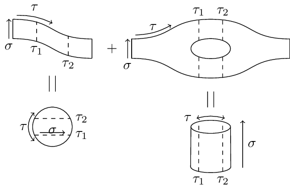
When calculating scattering amplitudes via the path integral, we must sum over all possible world-sheet topologies. To characterize the types of world-sheets that have to be considered at each level of its perturbative expansion, string theory makes use of the following theorem:
Every compact, connected, oriented two-dimensional manifold is topologically equivalent to a sphere with handles ( for genus) and boundaries. A topological invariant of two-dimensional oriented surfaces is the Euler characteristic .
What this boils down to is that we can obtain the topological characteristics of higher and higher loop-level world-sheet topologies by successively increasing in one-step increments the number of handles in case of the closed string and the number of boundaries for the open sector. This gives the topologies in this figure for the vacuum diagram of the closed sector up to one-loop level. For the closed sector, see closed string topologies.
Operator Orderings

Organic Molecule
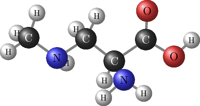
Beta-methylamino-DL-alanine - C4H10N2O2. Coordinates found on https://tex.stackexchange.com/q/453740.
Otto Cycle
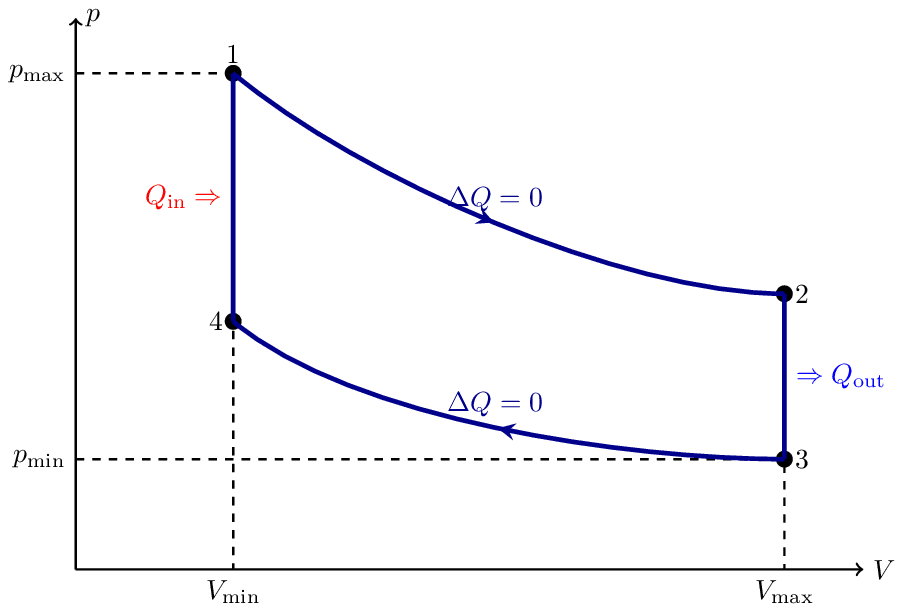
The Otto cycle is an idealized thermodynamic cycle of a typical spark ignition piston engine. It is the thermodynamic cycle most commonly found in automobile engines.
Periodic Table
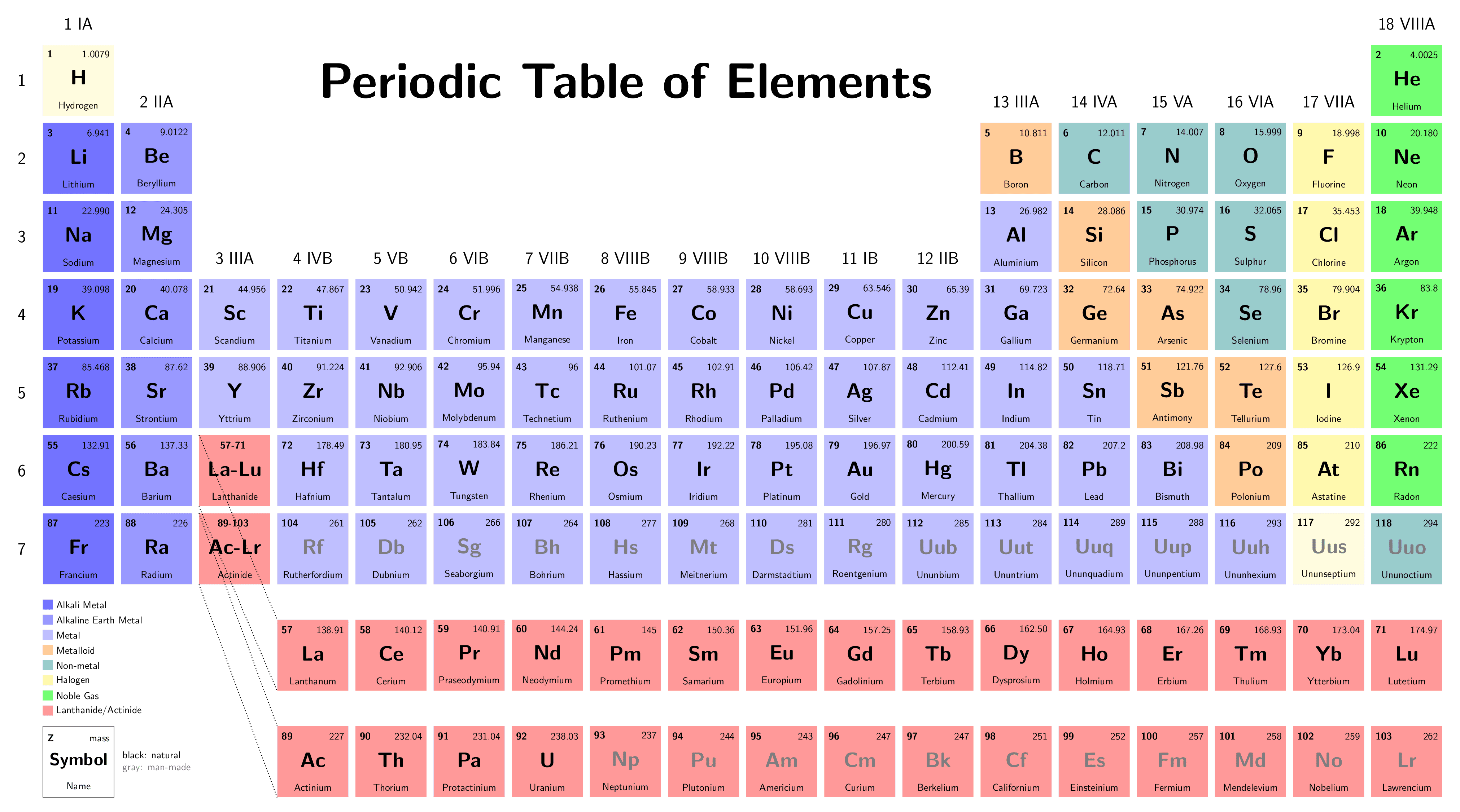
The periodic table of elements, a graphic formulation of the periodic dependence of elemental properties on their atomic numbers. The table is divided into four roughly rectangular areas called blocks. Rows are called periods, columns are groups. Elements from the same group show similar chemical characteristics. Trends run through the periodic table, with nonmetallic character (keeping their own electrons) increasing from left to right across a period, and from down to up across a group, and metallic character (surrendering electrons to other atoms) increasing in the opposite direction.
Physics Mindmap
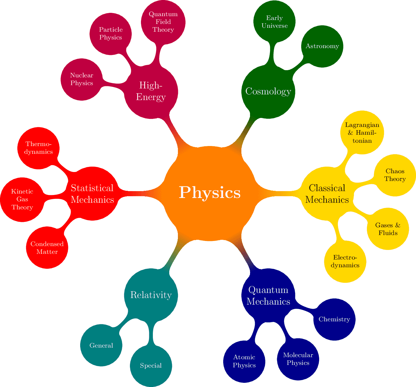
A mindmap showing the main branches of physics, including Classical Mechanics, Quantum Mechanics, Relativity, Statistical Mechanics, High-Energy Physics, and Cosmology. Each branch is further divided into subcategories.
Plane to Torus

Plate Capacitor
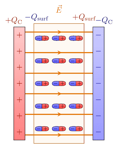
Parallel plate capacitor with dipolar polarization.
Poles
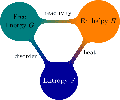
Potential Triangle
Propagator Fluctuations
Propagators
Random Forest
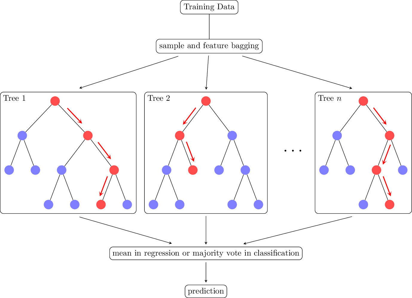
Diagram of the random forest (RF) algorithm (Breiman 2001). RFs are ensembles model consisting of binary decision trees that predicts the mode of individual tree predictions in classification or the mean in regression. Every node in a decision tree is a condition on a single feature, chosen to split the dataset into two so that similar samples end up in the same set. RFs are inspectable, invariant to scaling and other feature transformations, robust to inclusion of irrelevant features and can estimate feature importance via mean decrease in impurity (MDI).
Regular vs Bayes NN

Relation Space
RNVP
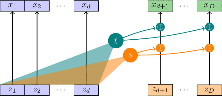
Illustration of the real-valued non-volume preserving (RNVP) affine coupling layer as introduced in arxiv:1605.08803. Inspired by https://blog.evjang.com/2018/01/nf2.html.
Roost Update

Representation Learning from Stoichiometry (Roost). Graph representation and update mechanism for the composition La2CuO4. Essentially depicting a graph convolution. arxiv:1910.00617
Sabatier Principle
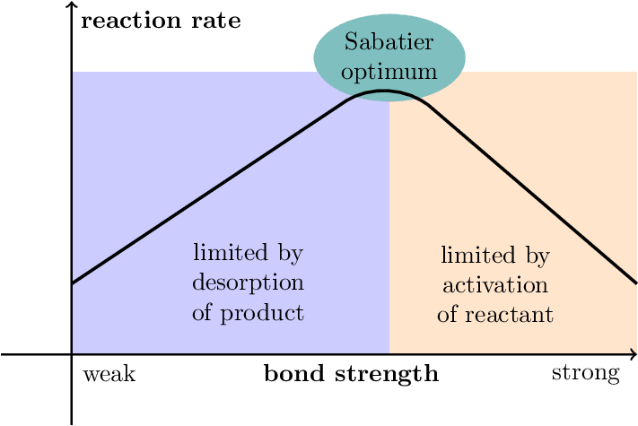
Illustration of the Sabatier principle in heterogeneous catalysis. Inspired by From the Sabatier principle to a predictive theory of transition-metal heterogeneous catalysis.
Saddle Point
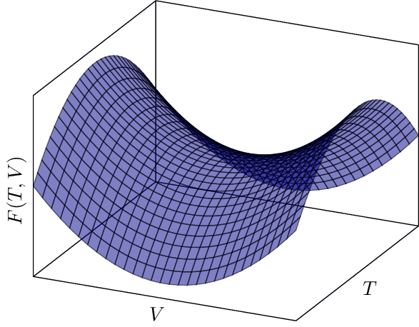
This graph depicts a saddle point in three-dimensional space, which is a point in the domain of a function that is a local minimum in one direction and a local maximum in another. The depicted function is quadratic in and , and the graph shows the convex and concave nature of the function along different axes.
Sbs Aktionen
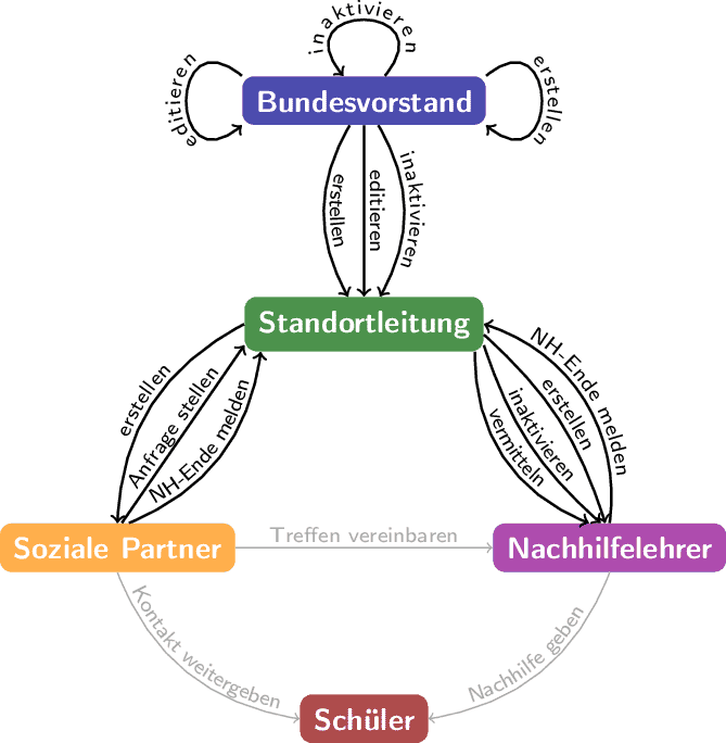
Operations schematic for the German student initiative "Studenten bilden Schüler eV". See https://studenten-bilden-schueler.de.
Scattering Process Detailed Balance

A simple diagram representing a scattering process in particle physics, where two incoming particles with momenta and interact and produce two outgoing particles with momenta and . The principle of detailed balance states that at equilibrium, each scattering process is in equilibrium with its reverse process.
Seebeck Effect
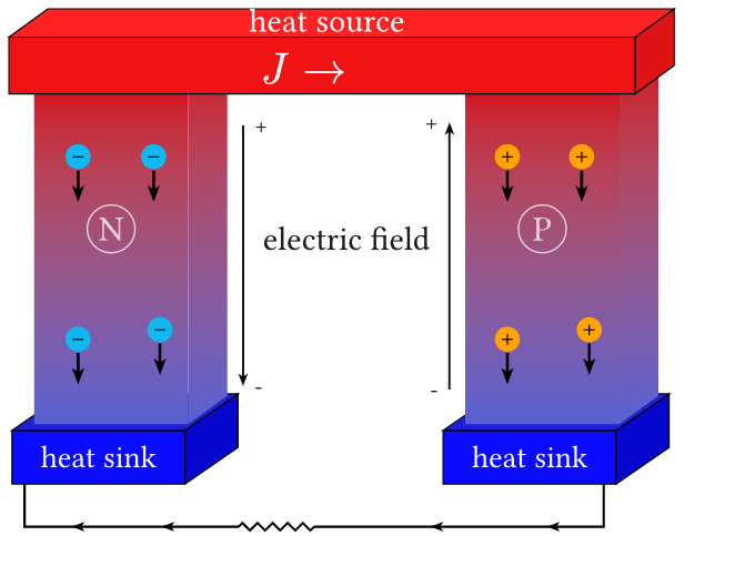
The Seebeck effect creates a voltage in conductors or semiconductor when subjected to a temperature gradient, i.e. when one side of the material is warmer than another. This effect enables thermoelectric devices which can measure temperature and generate electricity from waste heat.
Self Attention
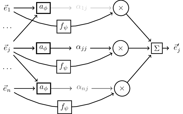
Illustrating the attention mechanism from arxiv:1706.03762.
Shell
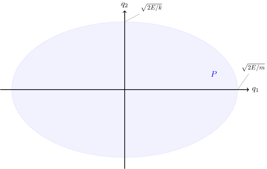
Sign Plane
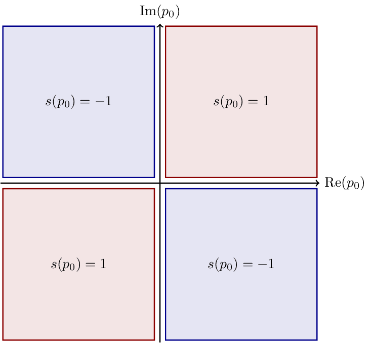
Sign function in the complex plane.
Single-head attention
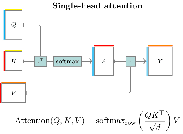
Flow diagram of single-head attention illustrating the equation with border colors to indicate tensor dimensions.
Skip Connection
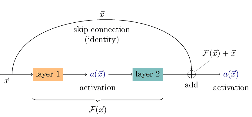
Illustration of skip connection in a residual block. Inspired by the ResNet paper. arxiv:1512.03385
Spider Diagram of Computational Methods in Materials Science
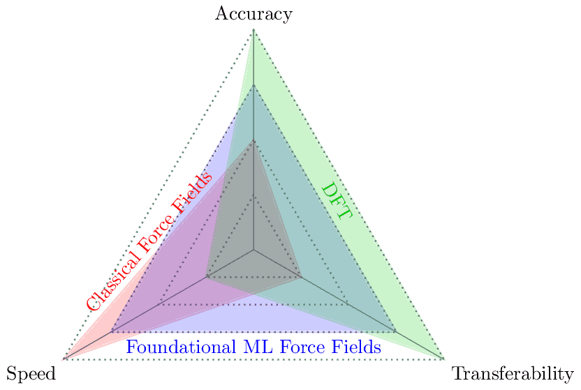
This spider diagram compares three computational chemistry methods: Classical Force Fields, Foundational ML Force Fields, and Density Functional Theory (DFT). The comparison is based on three key attributes:
- Accuracy: The precision and reliability of the method's predictions.
- Speed: The computational efficiency and time required for simulations.
- Generalizability: The ability to be applied across diverse chemical systems and material classes.
- Classical Force Fields (red): Highest speed, medium accuracy, lowest generalizability.
- DFT (green): Highest accuracy and generalizability, but lowest speed.
- Foundational ML Force Fields (blue): Balanced performance across all attributes, positioned between classical methods and DFT.
This diagram shows common trade-offs, highlighting how Foundational ML Force Fields aim to bridge the gap between the speed of classical methods and the accuracy of DFT, while offering improved generalizability over classical force fields.
Spontaneous Magnetization
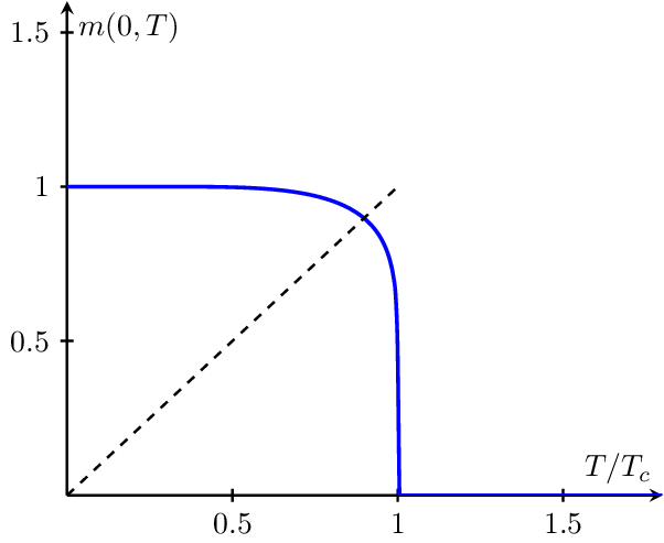
Spontaneous magnetization in an Ising ferromagnet appears below the critical temperature . The derivative of diverges in the limit .
Tanh
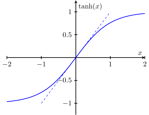
Plot of the hyperbolic tangent. tanh(x) goes to +/- 1 for x to +- infinity while it is approximately linear for abs(x) < 1. Appears in many places in physics, e.g. in the magnetization of an ideal paramagnet of independent spins.
Temperature-Dependent Phase Transition
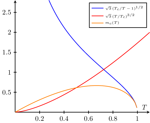
A plot illustrating the temperature-dependent phase transitions of a material as a function of the critical temperature (). The blue curve represents the low-temperature phase, the red curve represents the high-temperature phase, and the orange curve shows the critical mass () as a function of temperature. This visualization helps to understand the behavior of materials as they undergo phase transitions due to changes in temperature.
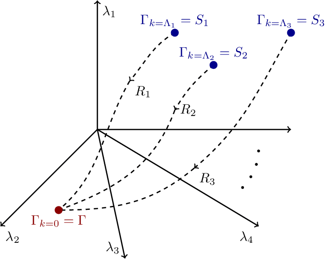
Theory Space
Thermodynamic Ensemble transforms

Equivalence of thermodynamic ensembles through Laplace and Legendre transforms.
Thomson Scattering
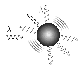
Illustration of coherent X-ray scattering (i.e. Thomson scattering) from an atom. An electron is caused to oscillate and then re-emits a photon with the same energy in an arbitrary direction.
Tori
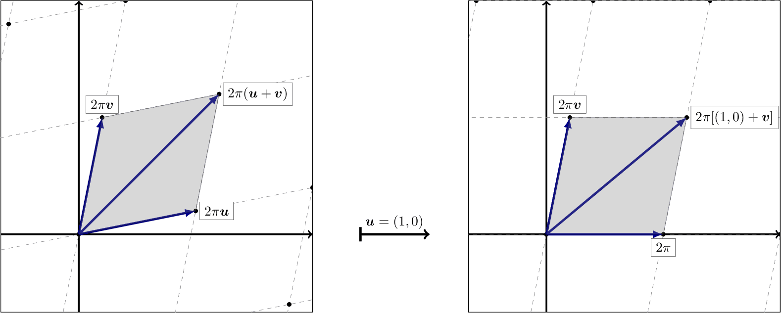
Torus
Torus Fundamental Domain
Two Point
Two-point propagator flow
Two Point No Cutoff
Two-point propagator flow without cutoff derivative
Unregularized Propagator Diagrams

VAE
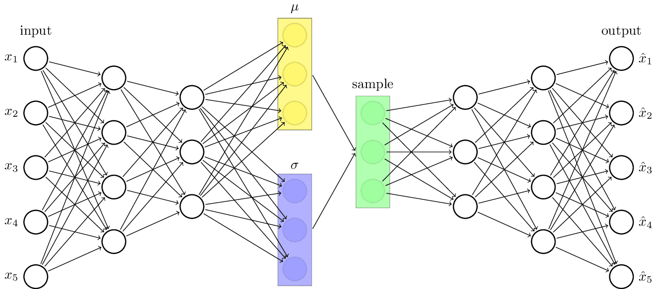
Variational autoencoder architecture. The earliest type of generative machine learning model. Inspired by https://towardsdatascience.com/intuitively-understanding-variational-autoencoders-1bfe67eb5daf.
Wall
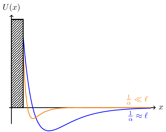
Exercise illustration: Compute the pressure of an ideal gas in three dimensions upon a wall at that attracts molecules at large distance and repels them at smaller distance. Let the force be given by the potential , with .
Wetterich Equation

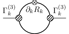
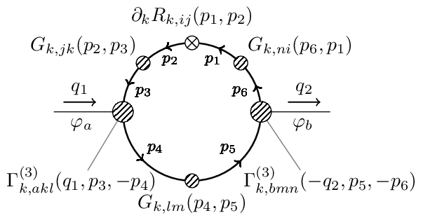
The Wetterich eqn. is a non-linear functional integro-differential equation of one-loop structure that determines the scale-dependence of the flowing action in terms of fluctuations of the fully-dressed regularized propagator . It admits a simple diagrammatic representation as a one-loop equation as shown in this diagram.
Wyckoff Positions
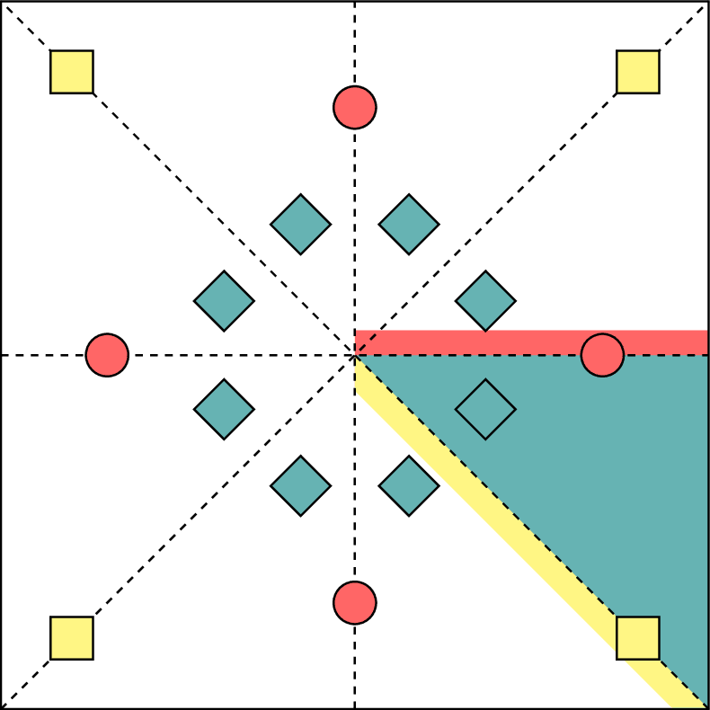
2D toy crystal with three occupied Wyckoff positions. The shaded areas illustrate the region of the unit cell the relevant atoms are constrained to lie in by specifying an anonymized Wyckoff position for that atom. Reproduction of fig. 2 from "Wyckoff Set Regression for Materials Discovery" by Rhys Goodall, inspired by PyXtal docs.
zT vs n
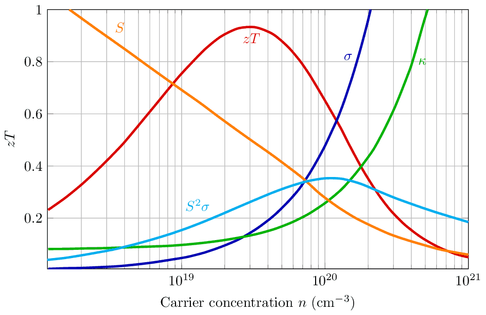
Thermoelectric figure of merit vs carrier concentration for Bi2Te3 based on empirical data in plot as a thermoelectric material performance indicator. Tuning for optimal involves a compromise between thermal conductivity , Seebeck coefficient and electrical conductivity . Increasing the electrical conductivity not only produces an increase in the electronic thermal conductivity but also usually decreases the Seebeck coefficient . This makes optimal difficult to achieve. Plot scales are , , .