Ferroelectric Response
Creator: Stefan Bringuier
Tags
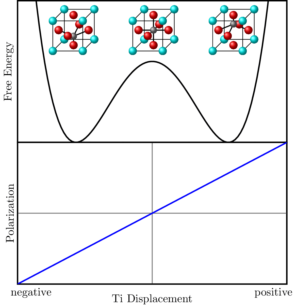
Schematic representation of ferroelectric response for BaTiO3 depicting the double-well free energy potential and polarization plots. The figure illustrates the movement of the Titanium atom within the crystal lattice as it shifts between two stable positions, corresponding to minima in the free energy curve. This Titanium displacement results in a large change in the material's polarization.
Edit
Download
Code
ferroelectric-response.tex (149 lines)
\documentclass{standalone}
\usepackage{tikz}
\usepackage{pgfplots}
\pgfplotsset{compat=1.18}
\usepgfplotslibrary{groupplots}
\usetikzlibrary{fadings,shadings,calc}

% Shape rendering specs
\pgfdeclareradialshading{atomshade}{\pgfpoint{0cm}{0cm}}{%
    color(0cm)=(pgftransparent!0);
    color(0.2cm)=(pgftransparent!20);
    color(0.5cm)=(pgftransparent!50);
    color(0.7cm)=(pgftransparent!70);
    color(1cm)=(pgftransparent!100)%
}

\tikzset{
    atom/.style={circle, shading=atomshade, minimum size=0.4cm},
    bond/.style={
        line width=0.5mm,
        shading=axis,
        color=black, %Change to #1 to specify bond color
        shading angle=45
    }
}

% Define BaTiO3 (#221) unit cell projection
\newcommand{\DrawUnitCell}[1]{%
    \begin{tikzpicture}[scale=1.5]
    % Draw the unit cell
    \draw[thick] (0,0,0) -- (1,0,0) -- (1,1,0) -- (0,1,0) -- cycle; % Bottom face
    \draw[thick] (0,0,1) -- (1,0,1) -- (1,1,1) -- (0,1,1) -- cycle; % Top face
    \draw[thick] (0,0,0) -- (0,0,1);
    \draw[thick] (1,0,0) -- (1,0,1);
    \draw[thick] (1,1,0) -- (1,1,1);
    \draw[thick] (0,1,0) -- (0,1,1);

    % Draw lines connect Oxygen to Titanium
    \begin{scope}
        \ifnum \pdfstrcmp{#1}{0.5} < 0
            % Connect bottom 4 oxygens to Ti
            \draw[bond=red] (0,0.5,0.5) -- ($(0,0.5,0.5)!0.5!(0.5,#1,0.5)$);
            \draw[bond=gray] ($(0,0.5,0.5)!0.5!(0.5,#1,0.5)$) -- (0.5,#1,0.5);
            \draw[bond=red] (1,0.5,0.5) -- ($(1,0.5,0.5)!0.5!(0.5,#1,0.5)$);
            \draw[bond=gray] ($(1,0.5,0.5)!0.5!(0.5,#1,0.5)$) -- (0.5,#1,0.5);
            \draw[bond=red] (0.5,0,0.5) -- ($(0.5,0,0.5)!0.5!(0.5,#1,0.5)$);
            \draw[bond=gray] ($(0.5,0,0.5)!0.5!(0.5,#1,0.5)$) -- (0.5,#1,0.5);
            \draw[bond=red] (0.5,0.5,0) -- ($(0.5,0.5,0)!0.5!(0.5,#1,0.5)$);
            \draw[bond=gray] ($(0.5,0.5,0)!0.5!(0.5,#1,0.5)$) -- (0.5,#1,0.5);
            \draw[bond=red] (0.5,0.5,1) -- ($(0.5,0.5,1)!0.5!(0.5,#1,0.5)$);
            \draw[bond=gray] ($(0.5,0.5,1)!0.5!(0.5,#1,0.5)$) -- (0.5,#1,0.5);
        \else
            \ifnum \pdfstrcmp{#1}{0.5} > 0
                % Connect top 4 oxygens to Ti
                \draw[bond=red] (0,0.5,0.5) -- ($(0,0.5,0.5)!0.5!(0.5,#1,0.5)$);
                \draw[bond=gray] ($(0,0.5,0.5)!0.5!(0.5,#1,0.5)$) -- (0.5,#1,0.5);
                \draw[bond=red] (1,0.5,0.5) -- ($(1,0.5,0.5)!0.5!(0.5,#1,0.5)$);
                \draw[bond=gray] ($(1,0.5,0.5)!0.5!(0.5,#1,0.5)$) -- (0.5,#1,0.5);
                \draw[bond=red] (0.5,1,0.5) -- ($(0.5,1,0.5)!0.5!(0.5,#1,0.5)$);
                \draw[bond=gray] ($(0.5,1,0.5)!0.5!(0.5,#1,0.5)$) -- (0.5,#1,0.5);
                \draw[bond=red] (0.5,0.5,1) -- ($(0.5,0.5,1)!0.5!(0.5,#1,0.5)$);
                \draw[bond=gray] ($(0.5,0.5,1)!0.5!(0.5,#1,0.5)$) -- (0.5,#1,0.5);
            \else
                % Connect 8 oxygens to form octahedron
                \draw[bond=red] (0,0.5,0.5) -- (1,0.5,0.5);
                \draw[bond=red] (0.5,0,0.5) -- (0.5,1,0.5);
                \draw[bond=red] (0.5,0.5,0) -- (0.5,0.5,1);
            \fi
        \fi
    \end{scope}

    % Draw the Oxygen atoms (Red) (back perspective)
    \node[atom, anchor=center,ball color=red] at (0,0.5,0.5) {};
    \node[atom, anchor=center,ball color=red] at (0.5,0,0.5) {};
    \node[atom, anchor=center,ball color=red] at (0.5,0.5,0.0) {};

    % Draw the Barium atoms (Cyan)
    \node[atom, anchor=center,ball color=cyan] at (0,0,0) {};
    \node[atom, anchor=center,ball color=cyan] at (1,0,0) {};
    \node[atom, anchor=center,ball color=cyan] at (0,1,0) {};
    \node[atom, anchor=center,ball color=cyan] at (1,1,0) {};
    \node[atom, anchor=center,ball color=cyan] at (0,0,1) {};
    \node[atom, anchor=center,ball color=cyan] at (1,0,1) {};
    \node[atom, anchor=center,ball color=cyan] at (0,1,1) {};
    \node[atom, anchor=center,ball color=cyan] at (1,1,1) {};

    % Titanium atom (Gray)
    \node[atom, anchor=center,ball color=gray, minimum size=0.25cm] at (0.5,#1,0.5) {};

    % Draw the Oxygen atoms (red) (front perspective)
    \node[atom, anchor=center,ball color=red] at (0.5,1,0.5) {};
    \node[atom, anchor=center,ball color=red] at (1,0.5,0.5) {};
    \node[atom, anchor=center,ball color=red] at (0.5,0.5,1) {};

    \end{tikzpicture}%
}

\begin{document}
\begin{tikzpicture}[scale=0.8]
    % Define top and bottom plots
    \begin{groupplot}[
        group style={group size=1 by 2, vertical sep=0pt},
        width=10cm,
        height=6cm,
        xtick=\empty,
        ytick=\empty,
        axis lines*=box,
        enlargelimits=false,
        xmin=-2.5, xmax=2.5,
        axis line style={very thick},
    ]
        % Double-well free energy potential
        \nextgroupplot[
            ylabel={Free Energy},
            ylabel style={rotate=0},
            ymin=0, ymax=3.5,
            xlabel={}, % Remove x-axis label from top plot
            tick style={draw=none},
        ]
        \addplot[domain=-2.5:2.5, samples=100, very thick] {0.5*(\x^4-4*\x^2+4)};

        % Polarization vs. displacement
        \nextgroupplot[
            ylabel={Polarization},
            ylabel style={rotate=-90},
            ymin=-2.5, ymax=2.5,
            xlabel={Ti Displacement},
            xlabel shift={-10pt},
            xlabel near ticks,
            ylabel near ticks,
            xtick={-2.25, 2.25},
            xticklabels={negative, positive},
            tick style={draw=none},
        ]
        % Additional axes through origin
        \draw[black!50, thick] (axis cs:0,-2.475) -- (axis cs:0,2.475);
        \draw[black!50, thick] (axis cs:-2.49,0) -- (axis cs:2.49,0);

        % Polarization line
        \addplot[domain=-2.5:2.5, samples=2, blue, very thick] {\x};
    \end{groupplot}

    % Overlay the unit cells manually
    \node[anchor=center] at (1.75,3.5) {\scalebox{0.5}{\DrawUnitCell{0.3}}};
    \node[anchor=center] at (4.25,3.5) {\scalebox{0.5}{\DrawUnitCell{0.5}}};
    \node[anchor=center] at (6.75,3.5) {\scalebox{0.5}{\DrawUnitCell{0.7}}};
\end{tikzpicture}
\end{document}