Open String Topologies
Tags
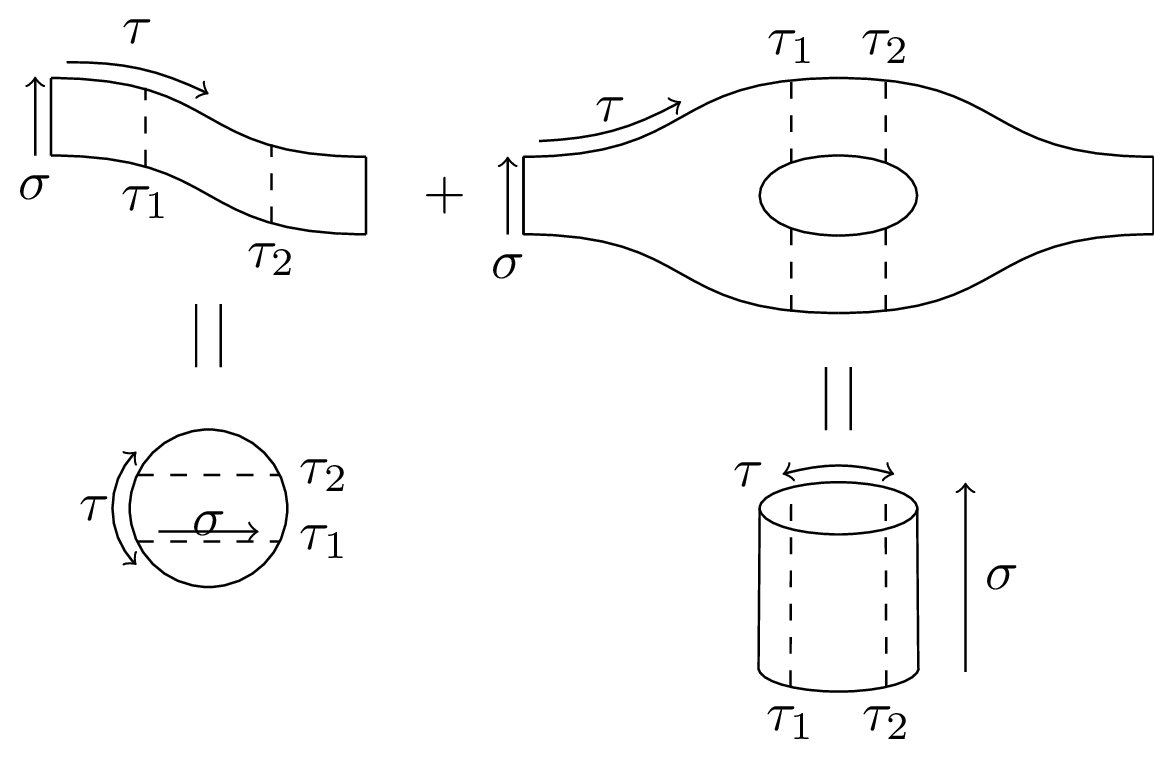
When calculating scattering amplitudes via the path integral, we must sum over all possible world-sheet topologies. To characterize the types of world-sheets that have to be considered at each level of its perturbative expansion, string theory makes use of the following theorem:
Every compact, connected, oriented two-dimensional manifold is topologically equivalent to a sphere with handles ( for genus) and boundaries. A topological invariant of two-dimensional oriented surfaces is the Euler characteristic .
What this boils down to is that we can obtain the topological characteristics of higher and higher loop-level world-sheet topologies by successively increasing in one-step increments the number of handles in case of the closed string and the number of boundaries for the open sector. This gives the topologies in this figure for the vacuum diagram of the closed sector up to one-loop level. For the closed sector, see closed string topologies.
Edit
Download
Code
open-string-topologies.tex (97 lines)
\documentclass[tikz]{standalone}

\usepackage{amsmath}
\usetikzlibrary{tqft,calc}

\begin{document}

\begin{tikzpicture}[
    every tqft/.append style={
        transform shape, rotate=90, tqft/circle x radius=7pt,
        tqft/circle y radius=0pt, tqft/boundary separation=1cm
      }
  ]

  % cobordism at upper left
  \pic[
    tqft/cylinder to prior,
    name=a,
    every outgoing lower boundary component/.style={draw},
    every incoming boundary component/.style={draw},
    cobordism edge/.style={draw},
  ];

  % annotation of cobordism at upper left
  \coordinate (temp1) at ($(a-incoming boundary.west)!0.3!(a-outgoing boundary.west) +(0,0.08)$);
  \coordinate (temp2) at ($(a-incoming boundary.west)!0.7!(a-outgoing boundary.west) +(0,-0.08)$);
  \draw[dashed]
  (temp1) node[below] {$\tau_1$} -- +(0,0.5)
  (temp2) node[below] {$\tau_2$} -- +(0,0.5);
  \draw[->] ($(a-incoming boundary.west) - (0.1,0)$) node[below] {$\sigma$} -- ++(0,0.5);
  \draw (a-outgoing boundary) ++(0.5,0) node {$+$};
  \draw[->] ($(a-incoming boundary.east)+(0.1,0.1)$) to[bend left=13] +(0.9,-0.2);
  \node[above] at ($(a-incoming boundary.east)+(0.55,0.1)$) {$\tau$};

  % cobordism at upper right consisting of two 'pants'
  \pic[
    tqft/pair of pants,
    name=b,
    every incoming upper boundary component/.style={draw},
    every incoming boundary component/.style={draw},
    cobordism edge/.style={draw},
    at={($(a-outgoing boundary)+(1,0)$)},
  ];

  \pic[
    tqft/reverse pair of pants,
    name=c,
    every outgoing lower boundary component/.style={draw},
    % every incoming boundary component/.style={draw},
    cobordism edge/.style={draw},
    at=(b-outgoing boundary 1),
  ];

  % annotation of cobordism at upper right
  \draw[->] ($(b-incoming boundary.west) - (0.1,0)$) node[below] {$\sigma$} -- ($(b-incoming boundary.east) - (0.1,0)$);
  \coordinate (temp1) at ($(b-between outgoing 1 and 2)!0.2!(c-between incoming 1 and 2) +(0,0.72)$);
  \coordinate (temp2) at ($(b-between outgoing 1 and 2)!0.8!(c-between incoming 1 and 2) +(0,0.72)$);
  \draw[dashed]
  (temp1) node[above] {$\tau_1$} -- +(0,-0.51) ++(0,-0.93) -- ++(0,-0.53)
  (temp2) node[above] {$\tau_2$} -- +(0,-0.51) ++(0,-0.93) -- ++(0,-0.53);
  \draw[->] ($(b-incoming boundary.east)+(0.1,0.1)$) to[bend right=13] +(0.9,0.25);
  \node[above] at ($(b-incoming boundary.east)+(0.55,0.1)$) {$\tau$};

  % drawing cylinder
  \path let \p1=(b-between outgoing 1 and 2), \p2=(c-between incoming 1 and 2) in
  node[name=cyl1, minimum width={\x2-\x1}] at ($(b-outgoing boundary 1)-(0,2.5)$) {}
  node[name=rec, shape=rectangle, minimum height=1cm, minimum width={\x2-\x1}, anchor=south]
  at (cyl1) {}
  node[name=cyl2, shape=ellipse, minimum height=.3cm, minimum width={\x2-\x1}, draw, outer sep=0]
  at (rec.north) {}
  ;
  \draw (cyl1.west) -- (cyl2.west) % left side
        (cyl1.east) -- (cyl2.east) % right side
        (cyl1.west) arc(-180:0:0.508cm and 0.15cm); % bottom ellipse

  % annotating cylinder
  \draw[<->] ($(cyl2.north east)+(0,0.1)$) to[bend right=15] ($(cyl2.north west)+(0,0.1)$);
  \node[left] at ($(cyl2.north west)+(0,0.1)$) {$\tau$};
  \draw[->] (cyl1.south east) ++ (0.3,0.1) -- ++(0,1.2);
  \draw (cyl1.south east) ++ (0.3,0.7) node [right] {$\sigma$};
  \draw[dashed] ($(cyl1.west)!0.2!(cyl1.east) +(0,-0.12)$) node[below] {$\tau_1$} --($(cyl2.west)!0.2!(cyl2.east) +(0,0.12)$)
  ($(cyl1.west)!0.8!(cyl1.east) +(0,-0.12)$) node[below] {$\tau_2$} --($(cyl2.west)!0.8!(cyl2.east) +(0,0.12)$);
  \draw (cyl2) ++(85:0.9) -- +(0,-0.4) (cyl2) ++(95:0.9) -- +(0,-0.4);
  % drawing and annotating circle
  \node[draw, shape=circle, minimum width=1cm]
  at (cyl2.west -| a-between first incoming and first outgoing) (circ) {};
  \draw[dashed] (circ) +(155:0.5) -- +(25:0.5) node[right] {$\tau_2$}
  +(205:0.5) -- +(335:0.5) node[right] {$\tau_1$};
  \draw[->] (circ) +(205:0.35) -- +(335:0.35);
  \node[below=-0.3em] at(circ) {$\sigma$};
  \draw (circ) ++(85:0.9) -- +(0,0.4) (circ) ++(95:0.9) -- +(0,0.4);
  \draw[<->] (circ.south west) +(-0.1,0) to[bend left=45] ($(circ.north west)+(-0.1,0)$);
  \node[left] at(circ.west) {$\tau$};
\end{tikzpicture}

\end{document}